Free-Vibration (Modal) Analysis

BeamAnalysis.modal() returns the natural frequencies and mode shapes of a beam. It assembles a consistent mass matrix alongside the stiffness matrix and solves the generalized eigenproblem

\[\mathbf{K}\,\boldsymbol\phi = \omega^2\,\mathbf{M}\,\boldsymbol\phi,\]

refining each span into nseg Euler–Bernoulli sub-elements so the higher modes are captured accurately. Supply the mass per unit length (in units consistent with EI); supports — including elastic springs — are taken from the beam, and the analysis is independent of any applied loads.

The result is a ModalResults carrying the frequencies (omega rad/s, f Hz, periods s) and the mode shapes, drawn with ``plot_results()`` (the beam schematic above the mode shapes) or ``plot_modes()`` (mode shapes only).

Supported for prismatic, fixed-fixed members without shear flexibility (GAv).

import numpy as np
import pandas as pd
import matplotlib.pyplot as plt
import pycba as cba

Example 1 - Simply-supported beam

For a prismatic simply-supported beam the natural circular frequencies are the standard textbook result

\[\omega_n = \left(\frac{n\pi}{L}\right)^2 \sqrt{\frac{EI}{\bar m}}.\]

We first evaluate this analytically, then obtain the same frequencies from PyCBA — keeping the two separate.

# Theory: the analytic natural frequencies
L, EI, mbar = 10.0, 1.0, 1.0          # length, EI, mass/length (consistent units)

n = np.arange(1, 5)
omega_exact = (n * np.pi / L) ** 2 * np.sqrt(EI / mbar)
f_exact = omega_exact / (2 * np.pi)
f_exact

array([0.01570796, 0.06283185, 0.14137167, 0.25132741])

Now solely the PyCBA usage — build the beam, supply the mass, and call modal(). plot_results() shows the mode shapes against the beam schematic:

# PyCBA: build the beam, run the modal analysis
modal = cba.BeamAnalysis([L], EI, [-1, 0, -1, 0]).modal(mass=mbar, n_modes=4)
print(modal)

modal.plot_results();

ModalResults(4 modes; f [Hz] = 0.01571, 0.06284, 0.1414, 0.2515)

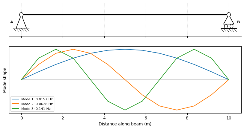
The computed frequencies match the analytic values closely:

pd.DataFrame(
    {"PyCBA f (Hz)": modal.f, "exact f (Hz)": f_exact},
    index=[f"mode {i}" for i in n],
).round(5)

	PyCBA f (Hz)	exact f (Hz)
mode 1	0.01571	0.01571
mode 2	0.06284	0.06283
mode 3	0.14141	0.14137
mode 4	0.25153	0.25133

Example 2 - Two-span continuous bridge

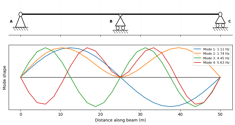
A two-span continuous bridge in SI units (N, m, kg). modal() returns omega (rad/s), f (Hz) and the natural periods (s); plot_results() shows the mode shapes against the bridge schematic — note the symmetric / antisymmetric pairs typical of a two-span deck.

E, I = 2.1e11, 1.4e-3          # Pa, m^4 (steel girder)
mbar_b = 1500.0                # kg/m (girder + deck)

bridge = cba.BeamAnalysis([25.0, 25.0], E * I, [-1, 0, -1, 0, -1, 0])
modal_b = bridge.modal(mass=mbar_b, n_modes=4)
for i in range(modal_b.n_modes):
    print(f"mode {i+1}:  f = {modal_b.f[i]:6.3f} Hz   (T = {modal_b.periods[i]:.3f} s)")

modal_b.plot_results(modes=[0, 1, 2, 3]);

mode 1:  f =  1.113 Hz   (T = 0.899 s)
mode 2:  f =  1.738 Hz   (T = 0.575 s)
mode 3:  f =  4.451 Hz   (T = 0.225 s)
mode 4:  f =  5.633 Hz   (T = 0.178 s)

Example 3 - Mesh density (nseg)

Each span is internally meshed into nseg Euler–Bernoulli sub-elements (default 12); one element per span would resolve only the first mode or two. The higher the mode, the finer the mesh it needs. Pass nseg= to control it — here we watch the 4th mode of the simply-supported beam of Example 1 converge to its analytic value as nseg increases (the consistent mass matrix approaches from above):

mode = 4
f4_exact = (mode * np.pi / L) ** 2 * np.sqrt(EI / mbar) / (2 * np.pi)

rows = []
for nseg in (2, 4, 8, 16, 32):
    f4 = cba.BeamAnalysis([L], EI, [-1, 0, -1, 0]).modal(mass=mbar, n_modes=4, nseg=nseg).f[3]
    rows.append((nseg, f4, 100 * (f4 / f4_exact - 1)))

df = pd.DataFrame(rows, columns=["nseg", "f4 (Hz)", "error (%)"]).set_index("nseg")
print(f"analytic f4 = {f4_exact:.5f} Hz")
df.round({"f4 (Hz)": 5, "error (%)": 2})

analytic f4 = 0.25133 Hz

	f4 (Hz)	error (%)
nseg
2	0.31958	27.16
4	0.27895	10.99
8	0.25232	0.39
16	0.25139	0.03
32	0.25133	0.00

Notes

• The mass is a mass per unit length, in units consistent with EI (e.g. kg/m with EI in N·m², giving frequencies in Hz).

• nseg (default 12) sets the sub-elements per span; the first several modes are already well within 1% with the default, while higher modes need a finer mesh (Example 3).

• plot_results() draws the beam schematic above the mode shapes; plot_modes() draws the mode shapes alone — both accept a modes= list and a units= argument.

• Supported for prismatic, fixed-fixed members without shear flexibility (GAv); elastic spring supports are included. Other combinations raise a clear NotImplementedError.