Defining Beams#
The beam configuration input data is to be in the following format:
Member Lengths (L)#
A vector of the lengths of each member.
Dimension: N x 1, where N is the number of members.
Units: m
Flexural Rigidity (EI)#
The flexural rigidity for each member.
A member may be prismatic (constant EI, given as a scalar) or
non-prismatic (variable EI). A non-prismatic member is defined with a
pycba.SectionEI object built from one or more contiguous segments that
together describe EI(x) over the span. x is the span-local physical
coordinate (0 at the span start, the real span length at the end). Segments
are added head-to-tail with add_segment(seg_type, x, ei, degree=None)
(chainable), or in one line by passing a list of specs to the constructor:
import pycba as cba
# Straight haunch -> flat soffit -> straight haunch over a 12 m span:
sec = (cba.SectionEI()
       .add_segment("linear", [0.0, 3.0], [3.0e5, 1.2e5])
       .add_segment("const",  [3.0, 9.0], 1.2e5)
       .add_segment("linear", [9.0, 12.0], [1.2e5, 3.0e5]))
The seg_type is one of:
"const"— constantEIover[x0, x1];x = [x0, x1],eiscalar."linear"— one linear piece;x = [x0, x1],ei = [ei0, ei1]."pwl"— piecewise-linear;x = [x0, …, xn](n ≥ 2 stations),eiof the same length, givingn − 1linear pieces with kinks at the interior stations."poly"— one polynomial piece;eiis either sample values (a polynomial of orderdegree, defaultlen(x) − 1, is fitted) or acallableei(x_local)evaluated in the span-local coordinate (e.g. a parabolic soffit,EI ∝ depth³).
Segments must be contiguous (each new segment’s x[0] equals the running
end; the first starts at 0) — gaps/overlaps raise an error — and the total
coverage must equal the span length. A coincident x carrying a different ei
across a join is an allowed step (discontinuous EI).
Non-prismatic members are analysed exactly by flexibility (force-method)
integration of the element stiffness, evaluated piece-by-piece between
consecutive breakpoints (segment joins and pwl kinks) so that kinks and
steps are captured exactly; a single const segment reproduces the closed-form
prismatic element to machine precision. Scalar and SectionEI members may be
freely mixed in the same beam.
Dimension: N x 1 (one scalar or SectionEI per span; a single value is
applied to all spans)
Units: kNm2
Restraints (R)#
A vector of restraints for each node, as defined by the ends of each member.
Each node has 2 degrees of freedom, vertical deflection and rotation, in that order, for each node.
Restraint for a degree of freedom is indicated by a “-1” value.
Unrestrained degrees of freedom are indicated by a “0” value.
Supports with a stiffness (kN/m or kNm/rad) are indicated by a positive value of the stiffness, k: i.e. “+k”
Dimension: 2N x 1
Units: kN/m or kNm/rad or None
Named supports (supports)#
Writing R by hand means tracking two DOFs per node and the -1/0/+k
convention. As a friendlier alternative, pass supports= instead of R= — a
list with one entry per node (left to right), each naming the support there:
Name(s) |
Meaning |
Lowers to |
|---|---|---|
|
pinned |
|
|
roller |
|
|
fully fixed |
|
|
free (e.g. a cantilever tip) |
|
Names are case-insensitive. The two letters e (encastre) and f (free) are
deliberately distinct so a built-in support is never confused with a free end.
In a beam, pin and roller are identical (there is no horizontal DOF to
distinguish them); both names are kept for readability. The same vocabulary
drives parse_beam_string (described under Element Types, below), so the two
entry points stay in lockstep.
# These two beams are identical:
ba = cba.BeamAnalysis(L=[7.5, 7.0], EI=30e4, supports=["p", "r", "r"])
ba = cba.BeamAnalysis(L=[7.5, 7.0], EI=30e4, R=[-1, 0, -1, 0, -1, 0])
An elastic spring carries a stiffness value, which a name cannot, so give
that node a raw [vertical, rotation] pair instead — this is also the general
escape hatch back to the R convention:
# Vertical spring (k = 5e4) at the middle node, rotation free:
ba = cba.BeamAnalysis(L=[7.5, 7.0], EI=30e4, supports=["p", [5e4, 0], "p"])
supports and R are mutually exclusive (pass one or the other), and
supports_to_R(supports) is available if you want the lowered vector directly.
An internal hinge is not a support — it is a moment release between two
members — so it cannot appear in supports; release the moment on the adjacent
member through its element type (FP/PF/PP; see Element Types, below)
instead.
If the restraints leave the structure under-supported, it is a mechanism —
the stiffness matrix is singular and the solution is meaningless. Before
solving, analyze() checks the free-DOF stiffness for this condition and
raises a clear ValueError rather than returning enormous, spurious
displacements:
ba = cba.BeamAnalysis([10.0], 30e4, R=[-1, 0, 0, 0])  # pin one end, free the other
ba.analyze()      # ValueError: Structure is geometrically unstable ... mechanism
This catches both insufficient supports and over-released internal hinges. You
can also test a model up front, without solving, via ba.is_stable() (which
returns a bool instead of raising). The result is cached per structure, so
looped analyses that vary only the loads (e.g. a moving-load run) incur the
check only once; it is re-evaluated only if the beam structure changes. For an
unusual but intentionally near-singular model you can skip it entirely with
ba.analyze(check_stability=False).
Load Matrix (LM)#
A List of Lists representing the applied loads.
Each entry is a single load descriptor whose length depends on the load type:
Type |
Name |
Format |
Columns |
|---|---|---|---|
1 |
UDL |
|
3 |
2 |
Point Load |
|
4 |
3 |
Partial UDL |
|
5 |
4 |
Moment Load |
|
4 |
5 |
Trapezoidal (full) |
|
4 |
5 |
Trapezoidal (partial) |
|
6 |
6 |
Imposed curvature |
|
3+ |
Load Types:
Uniformly Distributed Loads, which only have a load value.
Point Loads, located at
afrom the left end of the span.Partial UDLs, starting at
afor a distance ofc(i.e. the cover) where \(L \geq a + c\).Moment Load, located at
a.Trapezoidal Load, linearly varying from
w1tow2.Full span:
[span, 5, w1, w2]—w1at the left end,w2at the right end.Partial:
[span, 5, w1, w2, a, c]—w1at positiona,w2at positiona + c, where \(L \geq a + c\).
Imposed Curvature (initial-strain) load, applying a free curvature field \(\kappa(x) = k_0 + k_1 x + \dots\) along the member. On a statically-determinate span it induces no internal forces, only a free deflected shape; on a restrained or continuous structure its restraint generates real moments and reactions. This is the mechanism for applying creep, shrinkage and thermal curvatures (e.g. for prestressed-concrete time-dependent analysis).
Dimension: M rows (one per applied load), with 3 or more columns per row depending on load type.
Units: kN, kN/m, and metres.
Load Cases and Response Combinations#
For independent analyses and arbitrary additive combinations, add named cases
to a LoadCases collection. A LoadCase is one arrangement of loads that can
be analysed directly. A LoadCombination is a weighted superposition of those
cases. Envelopes are then formed from the extrema of analysed cases or
combinations.
This is the natural place to translate design-code action categories and
combination equations into analysis input: for example, a code may define
permanent (G) and variable (Q) actions with partial factors, combination
factors, and arrangement rules. PyCBA does not implement a design code directly;
it provides the load-case, factor and patterning machinery for applying the code
you choose.
A load case can be built from a raw load matrix, or by using higher-level load helpers:
load_cases = cba.LoadCases(beam)

load_cases.add_case("G").add_udl(1, 5.0).add_udl(2, 5.0)
load_cases.add_udl("Q1", 1, 10.0)
load_cases.add_pl("Q2", 2, 20.0, 3.0)
# A UDL over global beam coordinates is split at span boundaries.
load_cases.add_segment_udl("Q3", x0=3.0, x1=12.0, w=8.0)

x, y = load_cases.combine({"G": 1.2, "Q1": 1.5}, response="M")
Use a LoadCombination when a named factor set is useful:
combo = cba.LoadCombination("1.2G + 1.5Q1", {"G": 1.2, "Q1": 1.5})
x, y = combo.response(load_cases, response="M")
LM = combo.to_LM(load_cases)
To inspect or plot one factored combination as a normal beam analysis, use
analyze_combination and then the standard BeamAnalysis methods:
analysis = load_cases.analyze_combination({"G": 1.2, "Q1": 1.5})
analysis.plot_results()
For a UDL that may be placed on selected parts of the beam, make_patterned_udl
creates one basis load case per span segment. A target combination then selects
the segments that increase one selected load effect:
udl_basis = cba.make_patterned_udl(beam, w=10.0, n_segments=20)
hogging = udl_basis.target_combination(
    "Hogging at first internal support",
    x=beam.beam.mbr_lengths[0],
    sense="min",
    response="M",
)
x, M = hogging.response(udl_basis)
LM = hogging.to_LM(udl_basis)
Changing n_segments changes the discretisation used by both the generated
basis cases and any combinations selected from them.
This segmented selection is related to Kadane’s maximum-subarray algorithm. If
segments may be selected independently, the target combination is formed by
including every segment with an adverse contribution at the target coordinate.
If a future loading rule requires a single contiguous loaded length, the same
segment response vector can instead be searched with a Kadane-style contiguous
subarray step before forming the LoadCombination.
LoadCases is a lower-level response-matrix and linear-combination utility.
LoadPattern is the high-level design-patterning workflow for dead and live
load max/min factors. The combined load-cases and load-patterning tutorial
shows how code-style combinations and patterning rules fit together. Internally,
a LoadPattern can be treated as a generator of factored LoadCases.
Each LoadCase stores ordinary PyCBA load-matrix rows, so it can also be
passed to LoadPattern.set_dead_loads or LoadPattern.set_live_loads where a
raw load matrix would otherwise be used:
lp = cba.LoadPattern(beam)
lp.set_dead_loads(load_cases.case("G"), 1.35, 0.9)
lp.set_live_loads(load_cases.case("Q1"), 1.5, 0.0)

pattern_cases = lp.to_load_cases()
pattern_LM = lp.to_LM()
env = lp.analyze()
pattern_cases.names lists the generated pattern names. pattern_LM is a
dictionary from generated pattern name to the exact factored LM used for that
analysis, which is useful when debugging a patterning rule. For a single
generated case, use pattern_cases[i].name and pattern_cases[i].to_LM().
Prescribed Displacements (D)#
An optional vector of prescribed nodal displacements (settlements), one entry per degree of freedom.
Use None for DOFs where the displacement is unknown (the default), and a float for DOFs whose displacement is known (e.g. a support settlement).
Fixed supports (
R = -1) default to zero displacement unless overridden byD.Spring supports (
R > 0) can also have a prescribed displacement; in that case the spring force isk_s × δand is reported inbeam_results.Rs.Constraint: a DOF cannot simultaneously have a spring (
R > 0), a prescribed displacement (D[i] ≠ None), and a non-zero consistent nodal load — this combination is physically inconsistent andanalyze()will raise aValueError.
Dimension: 2N+2 x 1 (same length as R)
Units: m (vertical DOFs), rad (rotational DOFs)
Element Types (eleType)#
Each member can be one of several element types, depending on the presence of
hinges in the beam. The two letters read left end then right end (F =
fixed/continuous, P = pinned/released):
FF— fixed-fixed (the default)FP— fixed-pinned (moment released at the right end)PF— pinned-fixed (moment released at the left end)PP— pinned-pinned (released at both ends)
Note that at a hinge, only one of the members meeting at that node should have a pinned end.
An element type can be given as the integer index, as a MemberType enum
member, or as its case-insensitive name string — the three forms are
equivalent:
import pycba as cba
from pycba import MemberType

# a two-span beam with a fixed-pinned then a pinned-fixed member
cba.BeamAnalysis(L, EI, R, eletype=[2, 3])
cba.BeamAnalysis(L, EI, R, eletype=[MemberType.FP, MemberType.PF])
cba.BeamAnalysis(L, EI, R, eletype=["FP", "PF"])
When assembling a beam member by member, Beam.add_member names the type
directly:
beam = cba.Beam()
beam.add_member(5.0, EI, "FP")          # or MemberType.FP, or 2
beam.add_member(6.0, EI, MemberType.PF)
Dimension: N x 1
Units: N/A
Visualising the Beam and Loads#
Once a beam is configured it can be drawn as a structural schematic — the beam,
its supports, internal hinges and the applied loads — using either a native
matplotlib backend or a TikZ/stanli
backend for publication-quality LaTeX figures. These draw the model (unlike
BeamAnalysis.plot_results, which draws the bending-moment, shear and deflection
results), so the beam does not need to have been analysed.
The supports are inferred from the restraint vector R: the first
vertical-only support is drawn as a pin and the remainder as rollers, a
fully-fixed node as an encastre wall, and a positive (spring) stiffness as a
spring. Internal moment releases are read from eleType and drawn as hinges.
Native matplotlib#
Beam.plot() draws the schematic on labelled axes (distance along the beam) and
returns the matplotlib Axes for further customisation. The beam below
exercises every support type — an encastré (E), rollers (R), an internal
hinge (H) and a spring set directly on the restraint vector — together with a
UDL, a point load, a partial UDL and a moment:
import pycba as cba

(L, EI, R, eType) = cba.parse_beam_string("E6R6H6R6R")
R[6] = 2000.0  # node 3: vertical spring support (stiffness in kN/m)
beam = cba.Beam(
    L,
    EI,
    R,
    eletype=eType,
    LM=[
        [1, 1, 20],            # UDL on span 1
        [2, 2, 50, 3.0],       # point load on span 2
        [3, 3, 12, 1.0, 4.0],  # partial UDL on span 3
        [4, 4, 40, 3.0],       # moment on span 4
    ],
)

ax = beam.plot()            # supports, loads, magnitudes and node labels
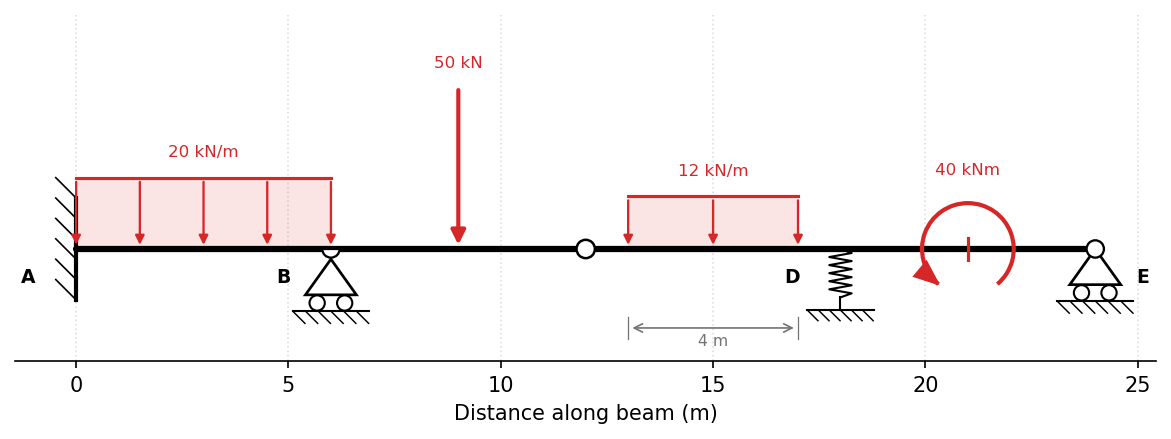
By default the matplotlib schematic relies on its x-axis for distance, so
span-length dimensions are off; pass dimensions=True to add them. Each
annotation is toggleable, and an existing Axes may be supplied:
beam.plot(ax=my_ax, dimensions=True)            # add span dimensions
beam.plot(labels=False, load_values=False)      # bare structure + loads
TikZ / stanli#
Beam.to_tikz() returns a standalone LaTeX document built on the stanli
package, and Beam.save_tikz() writes it to a file. With compile=True it is
rendered straight to PDF with pdflatex (which must be available, with the
stanli package installed):
tex = beam.to_tikz()                     # LaTeX source as a string
beam.save_tikz("beam.tex")               # write the .tex
beam.save_tikz("beam.tex", compile=True) # also produce beam.pdf
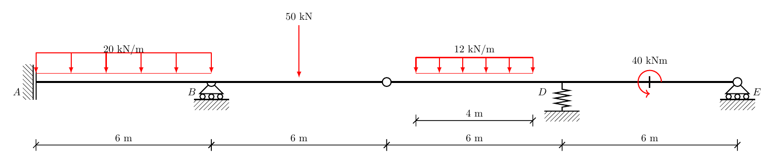
Pass standalone=False to emit just the tikzpicture environment for
embedding in a larger document.
Choosing what loads to draw#
By default the beam’s own load matrix is drawn. The loads argument (accepted
by plot, to_tikz and save_tikz) selects a different source, so the same
beam structure can be drawn with any loading — or none:
beam.plot()                 # the beam's own load matrix (default)
beam.plot(loads=[])         # the bare structure only
beam.plot(loads=[[1, 1, 10]])  # an explicit load matrix

# A high-level load case or factored combination
load_cases = cba.LoadCases(beam)
load_cases.add_case("G").add_udl(1, 5.0).add_udl(2, 5.0)
load_cases.add_pl("Q", 2, 20.0, 3.0)
beam.plot(load_cases.case("G"))

combo = cba.LoadCombination("ULS", {"G": 1.35, "Q": 1.5})
beam.plot(combo, load_cases=load_cases)   # draws the factored loads
The underlying pycba.render.BeamPlotter class is also available directly if
you want to build the renderer once and call both backends.
Units#
PyCBA is unit-agnostic: the solver performs no unit conversions, so any
internally consistent set of units may be used (e.g. kN, m, kNm — or N, mm,
N·mm) as long as every input shares the same system. Units surface only when a
result is plotted — in the axis labels and the deflection display scale —
and these are governed by a display unit system.
The default is SI with kN and m, matching PyCBA’s historical labels, so
nothing changes unless you ask for it. Choose a different system globally with
set_units:
cba.set_units("US-ft") # kip, ft, kip·ft; deflection shown in inches
or override it for a single figure with the units= argument accepted by every
plotting method (plot_results, Beam.plot, BridgeAnalysis.plot_static,
animate, …):
beam_analysis.plot_results(units="N-mm")
beam.plot(units="US-in")
bridge_analysis.plot_static(30.0, units="US-ft")
The built-in presets are:
Name |
Force |
Length |
Moment |
Deflection |
|---|---|---|---|---|
|
kN |
m |
kNm |
mm |
|
N |
mm |
N·mm |
mm |
|
kip |
ft |
kip·ft |
in |
|
kip |
in |
kip·in |
in |
|
— |
— |
— |
— |
"none" drops the unit labels entirely for a dimensionless presentation. For
anything else, build a pycba.units.UnitSystem directly and pass it wherever a
preset name is accepted:
from pycba.units import UnitSystem

mn_m = UnitSystem(
    name="MN, m", force="MN", length="m", moment="MN·m",
    distributed="MN/m", disp_label="mm", disp_scale=1000.0,
)
cba.set_units(mn_m)
Because this is a display layer only, the system you choose must match the
units of your inputs — PyCBA does not convert the numbers for you. The
deflection axis is the one place a number is rescaled for display
(disp_scale, e.g. ×1000 to show metres as millimetres).
Post-Tensioning (equivalent loads)#
A draped post-tensioning tendon can be turned into the equivalent (“balanced”)
loads it exerts on the concrete with the pycba.prestress preprocessor. It is
only a preprocessor: it returns an ordinary load matrix that you apply to the
beam like any other loading — the analysis itself is unchanged.
The tendon is described span by span by a profile whose geometry is given as eccentricities from the section centroid, positive below the centroid (so a sagging tendon balances gravity). The profiles mirror the standard library used by RAPT / PT Designer — 12 types, 7 for spans and 5 for cantilevers — via four profile objects:
Object |
RAPT/PT-Designer types |
Parameters (eccentricities + positions) |
|---|---|---|
|
1, 2 (8, 9 on cantilevers) |
|
|
3 |
|
|
4, 5 (10, 11 on cantilevers) |
|
|
6, 7 |
|
import pycba as cba
from pycba.prestress import Parabola, equivalent_loads

# a 2-span continuous beam
beam = cba.BeamAnalysis(L=[20.0, 20.0], EI=4.0e5, R=[-1, 0, -1, 0, -1, 0])

# a parabolic tendon: low at each midspan, raised over the interior support
F = 1500.0  # effective prestress force
loads = equivalent_loads(
    beam,
    force=F,
    profiles=[
        Parabola(e_left=0.0, e_mid=0.35, e_right=-0.25),  # span 1
        Parabola(e_left=-0.25, e_mid=0.35, e_right=0.0),  # span 2
    ],
)

beam.set_loads(loads)   # the balanced loads are now an ordinary loading
beam.analyze()
beam.plot_results()     # M here is the balanced moment M_bal
pycba.prestress.plot_tendon(beam, force, profiles) draws three stacked, x-aligned panels — the beam, the (exaggerated) cable drape, and the equivalent loads it produces — to show how the profile becomes the loading.
A cantilever (free-end) span is detected automatically and uses the cantilever form of its profile (the tendon anchors at the free tip).
The equivalent loads are generated from first principles from the piecewise
tendon e(x): a uniform load w = F·e″ over each parabolic segment, a point
load P = F·Δe′ at each interior kink, an anchorage moment F·e at each end,
and an anchorage force F·e′ at a free tip. Applying them gives the balanced
moment M_bal; the secondary (parasitic) moment is then M₂ = M_bal − F·e,
where e = e(x) is the tendon eccentricity.
The profile geometry and the equivalent-load derivation follow the standard PT references; see in particular the PT Designer Theory Manual, Chapters 5 (Tendon Profiles) and 6 (Equivalent Loads), available here, whose 12-profile library this preprocessor reproduces.
A worked, validated example follows Gilbert, Mickleborough & Ranzi (Design of Prestressed Concrete to AS3600-2009, Example 11.1) — see the Introduction tutorial.
Non-prismatic members. The equivalent transverse loads are the physical
curvature of the tendon (w = F·e″) and so are independent of the section, and
PyCBA analyses variable-EI members directly — so a draped tendon on a
non-prismatic beam (pass a SectionEI as EI) is handled correctly, including
its effect on the secondary moments. Eccentricities are taken from the beam
reference axis; for a non-prismatic section the concrete centroid moves within
the section, which matters for stress checks and the primary/secondary split
but not for the equivalent loads or M_bal.