ospgrid Educational

This tutorial illustrates some of the features that make ospgrid useful for education.

We start with the usual imports…

# Basic imports
import ospgrid as ospg  # The main package
from IPython import display  # For images in this notebook

# And just to make printed outputs easier to read
import numpy as np
np.set_printoptions(precision=2, suppress=True)

Example 1

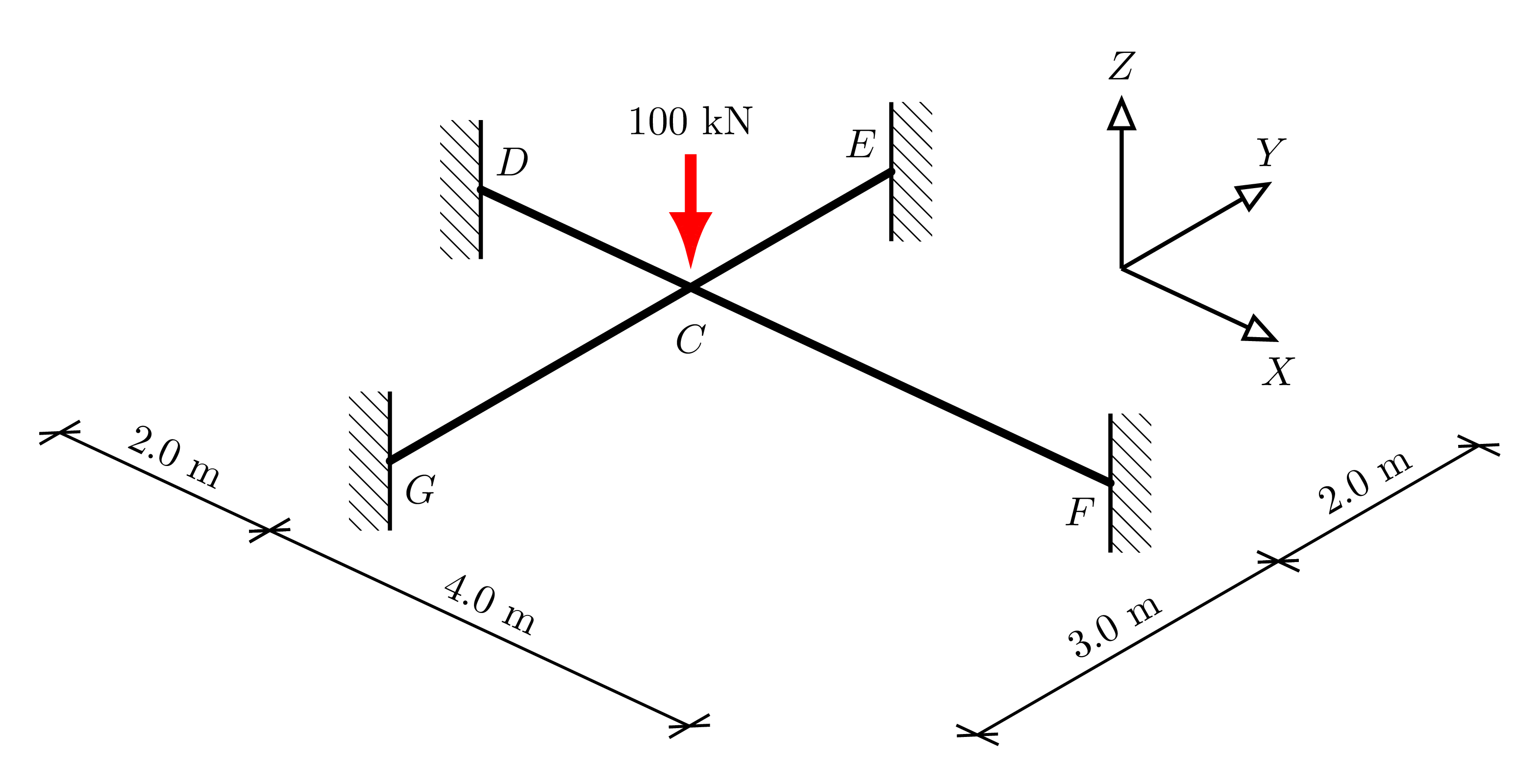
Here we use the Example 2 grid from CIV4280 Bridge Design & Assessment

display.Image("./images/edu_ex_1.png",width=800)

And quickly build the grid (see the Introduction tutorial for details):

grid = ospg.Grid()

grid.add_node("C", 0, 0)
grid.add_node("D", -2, 0)
grid.add_node("E", 0, 2)
grid.add_node("F", 4, 0)
grid.add_node("G", 0, -3)

EI = 200e9 * 50e6 / 1e15
GJ = 80e9 * 200e6 / 1e15
grid.add_member("C", "D", EI, GJ)
grid.add_member("C", "E", EI, GJ)
grid.add_member("C", "F", EI, GJ)
grid.add_member("C", "G", EI, GJ)

grid.add_load("C", Fz=-100)

grid.add_support("D", ospg.Support.FIXED)
grid.add_support("E", ospg.Support.FIXED)
grid.add_support("F", ospg.Support.FIXED)
grid.add_support("G", ospg.Support.FIXED)

osp = grid.analyze()

Notice that we have now returned the OpenSeesPy object osp created during the analysis - we will return to this.

Now the grid is analyzed and stored, we can examine aspects that should match the theory or a calculation.

Member Forces

Rather than just working off the plots, we can get the member end forces values. The DOFs are in the order translation about the \(x\)-, \(y\)-, and \(z\)-axes, and rotation about the \(x\)-, \(y\)-, and \(z\)-axes. With 6 DOFs per node, this is a \(12\times1\) vector, with the \(i\)-node and \(j\)-node as created (not necessarily as passed in the tuple):

Fcd = grid.get_member_forces(("C", "D"))
print(Fcd)

[  0.     0.   -34.85   4.61 -30.78   0.     0.     0.    34.85  -4.61
 -38.92   0.  ]

and as expected for grids, the forces in the \(x\) and \(y\) directions, and the moment about \(z\) are zero at each node.

Global Stifness Matrix

We can extract the reudced global stiffness matrix (i.e. after the boundary conditions have been applied). For this grid, only node \(C\) can move. Since OpenSeesPy uses a general 3D frame element, each node has 6 DOFs and so we will have a \(6\times6\) matrix in this instance.

Again, the DOFs are in the order translation about the \(x\)-, \(y\)-, and \(z\)-axes, and rotation about the \(x\)-, \(y\)-, and \(z\)-axes.

Of the 6 DOFs at node \(C\) here, because it is a grid, we know that the translations in \(x\) and \(y\), and the rotation about \(z\) will be zero.

As noted, OpenSeesPy uses a full 3D elastic frame element for its analysis. For hand analysis, we can suppress those DOFs we already know are not relevant, and so for grids we can work off stiffness matrices and force vectors corresponding to just translation in \(z\), and rotation about the \(x\)- and \(y\)-axes.

K = grid.get_system_stiffness()
print(K)

[[ 1944.45     0.       0.       0.       0.    -833.33]
 [    0.    1687.51     0.       0.       0.   -1125.  ]
 [    0.       0.   36319.44  8333.33 11250.       0.  ]
 [    0.       0.    8333.33 45333.33     0.       0.  ]
 [    0.       0.   11250.       0.   43333.33     0.  ]
 [ -833.33 -1125.       0.       0.       0.    6333.33]]

Member & Node Objects

While the use of the grid object gives access to the key outputs for an analysis, we can use the member and node objects to interrogate the underlying details. So let’s get the object for member \(CD\):

member_CD = grid.get_member(("C", "D"))

And it’s interesting to see what properties and methods are available in this object. Here we filter out the built-in methods for clarity:

[x for x in dir(member_CD) if not x.startswith('__')]

['EI',
 'GJ',
 'L',
 'delta_x',
 'delta_y',
 'get_global_stiffness',
 'get_local_stiffness',
 'get_transformation_matrix',
 'idx',
 'node_i',
 'node_j']

And so we can retrieve some member properties:

[member_CD.EI, member_CD.GJ, member_CD.L]

[10000.0, 16000.0, 2.0]

And get its node objects:

node_D = member_CD.node_j

which in turn have their own properties:

[x for x in dir(node_D) if not x.startswith('__')]

['Fz',
 'Mx',
 'My',
 'idx',
 'label',
 'set_load',
 'set_support',
 'support',
 'x',
 'y']

Adn for example, we can see the type of support assigned to node_D:

node_D.support

<Support.FIXED: [1, 1, 1, 1, 1, 1]>

The documentation explains the complete API in detail.

Member Stiffness Matrix (Local Coordinates)

The member stiffness matrix in the local coordinate system for a grid element (omitting the rows and columns corresponding to translations in \(x\) and \(y\) and rotation about \(z\)) is:

\[\begin{split}k = \left[ \begin{array}{cccccc} \dfrac{12EI}{L^3} & 0 & \dfrac{6EI}{L^2}& \dfrac{-12EI}{L^3}&0 & \dfrac{6EI}{L^2} \\[10pt] 0 & \dfrac{GJ}{L} & 0 & 0 & \dfrac{-GJ}{L} & 0 \\[10pt] \dfrac{6EI}{L^2} & 0 & \dfrac{4EI}{L} & \dfrac{-6EI}{L^2}&0 & \dfrac{2EI}{L} \\[10pt] \dfrac{-12EI}{L^3} & 0 & \dfrac{-6EI}{L^2} & \dfrac{12EI}{L^3}&0 & \dfrac{-6EI}{L^2} \\[10pt] 0 & \dfrac{-GJ}{L} & 0 & 0 & \dfrac{GJ}{L} & 0 \\[10pt] \dfrac{6EI}{L^2} & 0 & \dfrac{2EI}{L} & \dfrac{-6EI}{L^2}&0& \dfrac{4EI}{L} \\[10pt] \end{array} \right]\end{split}\]

We can retrieve this for member \(CD\) as follows:

k_eb = member_CD.get_local_stiffness()
print(k_eb)

[[ 15000.      0.  15000. -15000.      0.  15000.]
 [     0.   8000.      0.      0.  -8000.      0.]
 [ 15000.      0.  20000. -15000.      0.  10000.]
 [-15000.      0. -15000.  15000.      0. -15000.]
 [     0.  -8000.      0.      0.   8000.      0.]
 [ 15000.      0.  10000. -15000.      0.  20000.]]

Member Stiffness Matrix (Global Coordinates)

The coordinate transformation matrix for a grid element is:

\[\begin{split}T = \left[ \begin{array}{cccccc} 1 & 0 & 0 & 0 & 0 & 0 \\[10pt] 0 & C & S & 0 & 0 & 0 \\[10pt] 0 & -S & C & 0 & 0 & 0 \\[10pt] 0 & 0 & 0 & 1 & 0 & 0 \\[10pt] 0 & 0 & 0 & 0 & C & S \\[10pt] 0 & 0 & 0 & 0 & -S & C \\[10pt] \end{array} \right]\end{split}\]

where the direction cosines are:

\[C = \frac{x_j - x_i}{L} \hskip{1cm} S = \frac{y_j - y_i}{L}\]

and with this definition, the member stiffness matrix in the global coordinates is given by:

\[K_g = T^T K T\]

Note that in the Direct Stiffness Method, the transofrmation matrix is not explicitly evaluated, but the resulting stiffness terms are summed with the contributions of other members to yield those in \(K_g\).

T = member_CD.get_transformation_matrix()
print(T)

[[ 1.  0.  0.  0.  0.  0.]
 [ 0. -1.  0.  0. -0.  0.]
 [ 0. -0. -1.  0. -0. -0.]
 [ 0.  0.  0.  1.  0.  0.]
 [ 0. -0.  0.  0. -1.  0.]
 [ 0. -0. -0.  0. -0. -1.]]

And the resulting member stiffness matrix in global coordinates is then:

Kg = member_CD.get_global_stiffness()
print(Kg)

[[ 15000.      0. -15000. -15000.      0. -15000.]
 [     0.   8000.      0.      0.  -8000.      0.]
 [-15000.      0.  20000.  15000.      0.  10000.]
 [-15000.      0.  15000.  15000.      0.  15000.]
 [     0.  -8000.      0.      0.   8000.      0.]
 [-15000.      0.  10000.  15000.      0.  20000.]]

OpenSeesPy object

As noted, ospgrid.grid.analyze() returns the OpenSeesPy object of the analysis. Any of its methods can be used to interrogate the analysis further.

For example, the system’s residual force vector at the end of the first analysis step should be zero for an linear elastic and geometrical analysis, and it can be found using the OpenSeesPy printB command:

osp.printB('-ret')

[0.0,
 0.0,
 -1.4210854715202004e-14,
 3.552713678800501e-15,
 5.329070518200751e-15,
 0.0]

Example 2

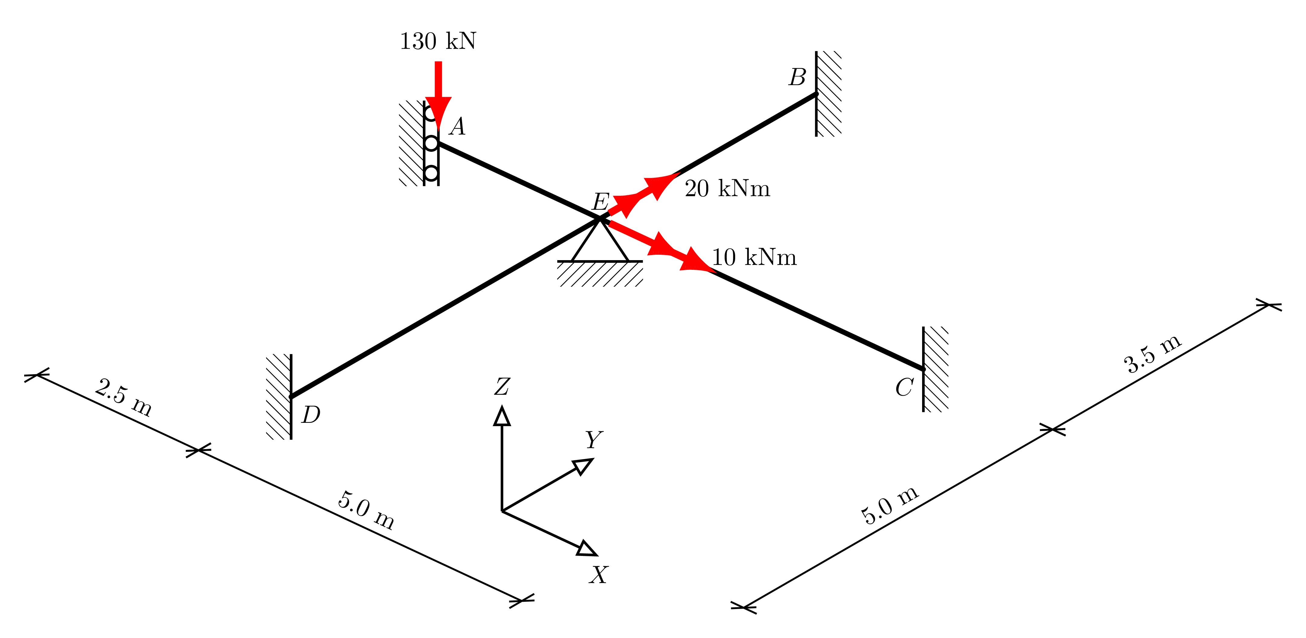
Returning to Example 2 from the Introduction to ospgrid, we will further illustrate the DOFs of the global stiffnes matrix.

display.Image("./images/intro_ex_2.png",width=800)

First, quickly create the grid:

grid = ospg.Grid()

grid.add_node("A", -2.0, 0.0)
grid.add_node("B", 0.0, 4.75)
grid.add_node("C", 4.0, 0.0)
grid.add_node("D", 0.0, -4.0)
grid.add_node("E", 0.0, 0.0)

EI = 10e3
GJ = 5e3
grid.add_member("A", "E", EI, GJ)
grid.add_member("B", "E", EI, GJ)
grid.add_member("C", "E", EI, GJ)
grid.add_member("D", "E", EI, GJ)

grid.add_load("E", Fz=-90, Mx=30, My=60)

grid.add_support("B", ospg.Support.FIXED)
grid.add_support("C", ospg.Support.FIXED)
grid.add_support("D", ospg.Support.FIXED)

osp = grid.analyze()

Now extract the reudced global stiffness matrix (i.e. after the boundary conditions have been applied):

K = grid.get_system_stiffness()
print(K)

[[   299.48      0.        0.        0.        0.      109.07     -0.
       0.        0.        0.        0.        0.  ]
 [     0.     1687.5       0.        0.        0.    -1125.        0.
   -1500.        0.        0.        0.    -1500.  ]
 [     0.        0.    19869.7   -1090.72  11250.        0.        0.
       0.   -15000.        0.    15000.        0.  ]
 [     0.        0.    -1090.72  22171.05      0.        0.        0.
       0.        0.    -2500.        0.        0.  ]
 [     0.        0.    11250.        0.    32302.63      0.        0.
       0.   -15000.        0.    10000.        0.  ]
 [   109.07  -1125.        0.        0.        0.     4842.11      0.
    1500.        0.        0.        0.     1000.  ]
 [    -0.        0.        0.        0.        0.        0.        0.
       0.        0.        0.        0.        0.  ]
 [     0.    -1500.        0.        0.        0.     1500.        0.
    1500.        0.        0.        0.     1500.  ]
 [     0.        0.   -15000.        0.   -15000.        0.        0.
       0.    15000.        0.   -15000.        0.  ]
 [     0.        0.        0.    -2500.        0.        0.        0.
       0.        0.     2500.        0.        0.  ]
 [     0.        0.    15000.        0.    10000.        0.        0.
       0.   -15000.        0.    20000.        0.  ]
 [     0.    -1500.        0.        0.        0.     1000.        0.
    1500.        0.        0.        0.     2000.  ]]

Since only nodes \(A\) and \(E\) can move, and all 6 DOFs are free at each, we obtain a \(12\times12\) matrix. From before, we know the DOFs are in the order translation about the \(x\)-, \(y\)-, and \(z\)-axes, and rotation about the \(x\)-, \(y\)-, and \(z\)-axes. Due to the suppoort conditions, we see entries in the rows/columns corresponding to DOFs \(\delta_{xA}\), \(\theta_{xE}\), \(\theta_{yE}\).